Introduction to PhiSpace
Annotating single cells with a bulk reference
Jiadong Mao
2026-10-13
Source:vignettes/PhiSpace.Rmd
PhiSpace.RmdIntroduction
PhiSpace annotates the cells of a query dataset with the phenotypes of an annotated reference, such as cell types or differentiation stages. It fits a partial least squares (PLS) regression of the reference phenotypes on gene expression, and then predicts a score for every phenotype in every query cell. These PhiSpace scores are continuous: a cell can score highly for two related phenotypes, which describes a transitional state better than a single label. The scores of a cell, one per phenotype, are its coordinates in the phenotype space.
The reference and the query can come from different technologies. In this vignette the reference is bulk microarray data of sorted mouse blood stem and progenitor cells from the Immunological Genome Project (ImmGen), and the query is single-cell RNA-seq of the same compartment (Nestorowa et al., 2016). The query cells were sorted with fluorescence-activated cell sorting (FACS) into known gates, so we can compare the PhiSpace scores with the FACS labels.
The method is described in Mao et al. (2025), Genome Biology
26, 323 (https://doi.org/10.1186/s13059-025-03755-8). The spatial
vignette, vignette("PhiSpaceST", package = "PhiSpace"),
applies PhiSpace to spatial transcriptomics. Larger case studies are on
the PhiSpace
website.
Installation
if (!requireNamespace("BiocManager", quietly = TRUE))
    install.packages("BiocManager")
BiocManager::install("PhiSpace")Data
Reference: ImmGen stem and progenitor cells
The ImmGen reference in celldex
contains 830 bulk microarray samples of sorted mouse immune cells. We
keep the 36 samples of stem and progenitor cells. Their labels
(label.fine) name the sorted populations, for example
LTHSC and SC.LT34F (long-term haematopoietic
stem cells), SC.MEP (megakaryocyte-erythroid progenitors),
SC.CMP.DR (common myeloid progenitors), GMP
(granulocyte-monocyte progenitors), MLP (multi-lymphoid
progenitors) and proB.CLP (common lymphoid
progenitors).
immgen <- fetchReference("immgen", "2024-02-26")
immgen <- immgen[, immgen$label.main == "Stem cells"]
reference <- SingleCellExperiment(
    assays = list(logcounts = as.matrix(assay(immgen, "logcounts"))),
    colData = colData(immgen)
)
reference$stage <- sub("^Stem cells \\((.*)\\)$", "\\1", reference$label.fine)
table(reference$stage)
#>
#>            GMP          LTHSC            MLP       proB.CLP SC.CD150-CD48-
#>              3              3              7              1              1
#>         SC.CDP      SC.CMP.DR       SC.LT34F         SC.MDP         SC.MEP
#>              3              2              3              3              2
#>      SC.MPP34F       SC.ST34F        SC.STSL
#>              2              2              4
Query: single-cell RNA-seq of stem and progenitor cells
The Nestorowa dataset in scRNAseq
contains 1,920 mouse stem and progenitor cells sequenced with
Smart-seq2. The column broad holds the FACS gate of each
cell; we keep the cells that have one. The genes are Ensembl
identifiers, so we map them to the gene symbols of the reference with
org.Mm.eg.db.
query <- fetchDataset("nestorowa-hsc-2016", "2024-04-18")
query <- query[, !is.na(query$broad)]
symbols <- AnnotationDbi::mapIds(
    org.Mm.eg.db::org.Mm.eg.db, keys = rownames(query),
    column = "SYMBOL", keytype = "ENSEMBL"
)
keep <- !is.na(symbols) & !duplicated(symbols)
query <- query[keep, ]
rownames(query) <- symbols[keep]
table(query$broad)
#>
#>   CMP   GMP  LMPP LTHSC   MEP   MPP
#>   328   123   280   323   362   368
Normalisation
PhiSpace needs the reference and the query to be normalised in the
same way. Here they are measured by different technologies, microarray
and single-cell RNA-seq, so we rank the genes within each sample with
RankTransf(). Ranks remove most differences of scale
between the two technologies. We first keep the genes measured in both
datasets.
genes <- intersect(rownames(reference), rownames(query))
length(genes)
#> [1] 18482
reference <- RankTransf(reference[genes, ], "logcounts", sparse = FALSE)
query <- logNormTransf(query[genes, ])
query <- RankTransf(query, "logcounts")
Annotation
PhiSpace() fits the PLS model on the reference and
stores the scores of the query cells in
reducedDim(query, "PhiSpace"). The argument
phenotypes names the reference column to predict, and
refAssay the assay to use (the query uses the same assay by
default). The number of PLS components, ncomp, controls the
complexity of the model; a good default is the number of phenotype
labels, here 13.
query <- PhiSpace(
    reference, query,
    phenotypes = "stage", refAssay = "rank", ncomp = 13
)
scores <- normPhiScores(reducedDim(query, "PhiSpace"))
dim(scores)
#> [1] 1784   13
normPhiScores() centres the scores of each phenotype at
their median and scales them to a maximum absolute value of 1, so that
the scores of different phenotypes are comparable.
Results
Scores by FACS gate
Each query cell has a score for each of the 13 reference stages. The heatmap shows the scores of all cells, grouped by their FACS gate.
gates <- c("LTHSC", "MPP", "LMPP", "CMP", "GMP", "MEP")
plotPhiSpaceHeatMap(
    scores,
    queryLabs = query$broad,
    queryLvls = gates,
    cluster_columns = TRUE,
    name = "Score"
)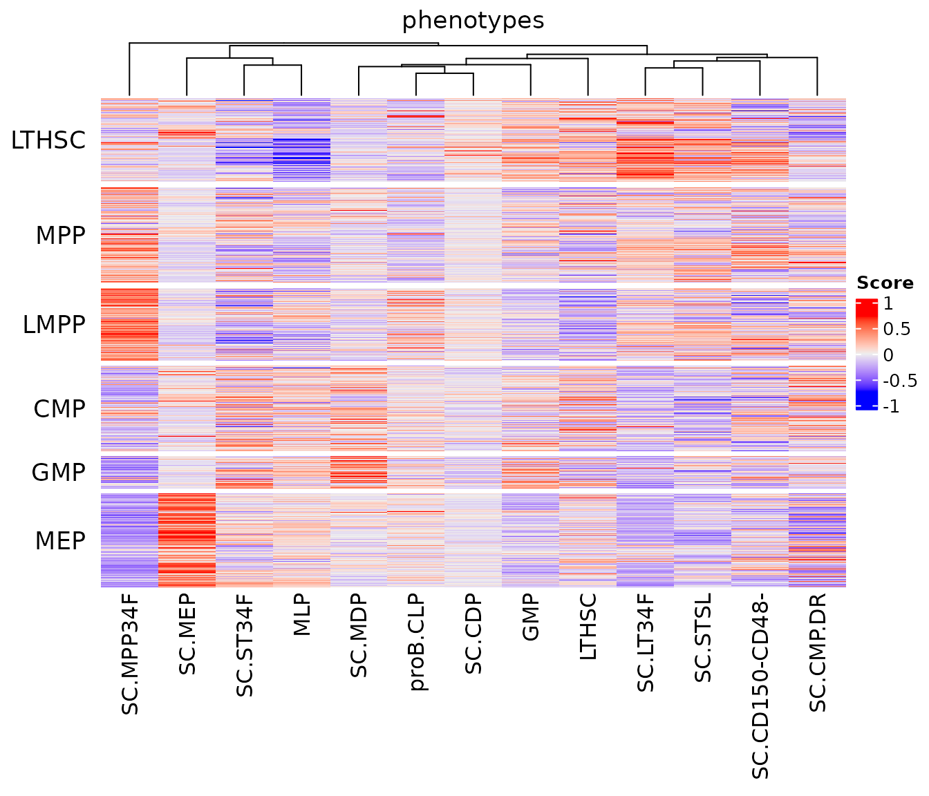
The mean score of each stage within each FACS gate summarises the heatmap.
gateMeans <- vapply(
    gates,
    function(g) colMeans(scores[query$broad == g, , drop = FALSE]),
    numeric(ncol(scores))
)
round(t(gateMeans), 2)
#>       SC.STSL SC.CD150-CD48- proB.CLP SC.LT34F SC.MDP SC.MEP SC.MPP34F SC.ST34F
#> LTHSC    0.21           0.08    -0.02     0.34  -0.06   0.02      0.03    -0.14
#> MPP      0.06           0.04    -0.03     0.07  -0.01  -0.03      0.24     0.03
#> LMPP     0.08           0.02     0.10     0.06  -0.04  -0.05      0.41    -0.15
#> CMP     -0.14          -0.03     0.03    -0.11   0.13   0.04     -0.09     0.12
#> GMP     -0.04          -0.04     0.05    -0.18   0.33   0.00     -0.26     0.12
#> MEP     -0.11          -0.04     0.03    -0.17   0.01   0.46     -0.28     0.02
#>       SC.CDP SC.CMP.DR   GMP   MLP LTHSC
#> LTHSC   0.09     -0.06  0.16 -0.32  0.14
#> MPP     0.01      0.01  0.01 -0.06 -0.03
#> LMPP    0.03      0.03 -0.07 -0.03 -0.18
#> CMP    -0.02      0.12  0.03  0.09  0.08
#> GMP    -0.08      0.05  0.17  0.10  0.02
#> MEP    -0.03     -0.09 -0.13  0.07  0.02
On average, cells sorted as MEP score highest for the ImmGen MEP
sample (SC.MEP), and cells sorted as long-term stem cells
(LTHSC) score highest for the long-term stem cell sample
SC.LT34F. The MPP and LMPP gates score highest for the
multipotent progenitor sample SC.MPP34F. The GMP gate
scores highest for SC.MDP (macrophage-dendritic cell
progenitors) and next for GMP; both are myeloid
progenitors. The CMP gate has no single top stage: its mean scores for
SC.MDP, SC.CMP.DR and SC.ST34F
are similar.
Discrete labels
A discrete label for each cell is the stage with the highest score. The table compares these labels with the FACS gates.
topStage <- colnames(scores)[max.col(scores, ties.method = "first")]
table(FACS = query$broad, PhiSpace = topStage)
#>        PhiSpace
#> FACS    GMP LTHSC MLP proB.CLP SC.CD150-CD48- SC.CDP SC.CMP.DR SC.LT34F SC.MDP
#>   CMP    13    30  26       12             22      2        66        2     61
#>   GMP    17     7   1        0              9      0        12        1     52
#>   LMPP    1     4   9       13             23      1        19       10      1
#>   LTHSC  10    31   3       16             22      5        11      124      0
#>   MEP     1    16   9        3             11      0        63        3      1
#>   MPP    13    21  11       10             54      2        27       17     10
#>        PhiSpace
#> FACS    SC.MEP SC.MPP34F SC.ST34F SC.STSL
#>   CMP       21        21       48       4
#>   GMP        4         3       14       3
#>   LMPP       1       167        9      22
#>   LTHSC     28        12       12      49
#>   MEP      239         2       11       3
#>   MPP        2       113       47      41
Discrete labels hide gradual differences between stages. For example, the 368 cells of the MPP gate have four common top stages, all early ones: SC.MPP34F (113 cells), SC.CD150-CD48- (54 cells), SC.ST34F (47 cells), SC.STSL (41 cells). The scores keep this information, because each cell has a score for every stage.
The phenotype space
A principal component analysis (PCA) of the scores shows the cells in
the phenotype space. getPC() returns the principal
component scores and the proportion of variance that each component
explains.
pc <- getPC(scores, ncomp = 3)
round(pc$props, 2)
#> [1] 0.31 0.16 0.12
pcDat <- data.frame(pc$scores, gate = factor(query$broad, levels = gates))
ggplot2::ggplot(pcDat, ggplot2::aes(comp1, comp2, colour = gate)) +
    ggplot2::geom_point(size = 0.8) +
    ggplot2::labs(x = "PC1", y = "PC2", colour = "FACS gate") +
    ggplot2::theme_bw()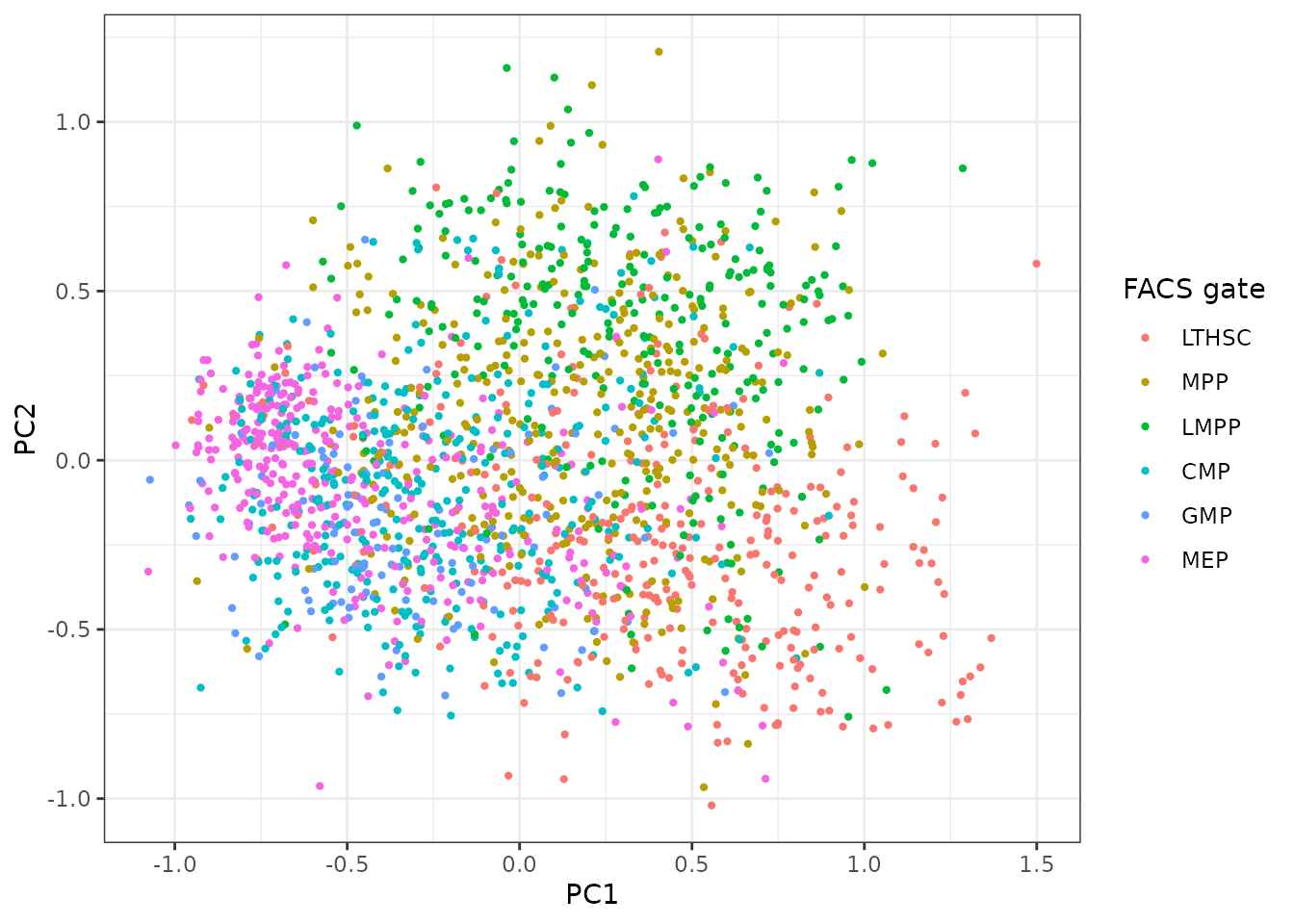
The first principal component orders the cells from the long-term stem cell gate to the MEP gate, and the second separates the LMPP gate from the others. The FACS gates overlap in the phenotype space, as expected for cells that differentiate gradually.
Session information
sessionInfo()
#> R version 4.5.0 (2025-04-11)
#> Platform: x86_64-pc-linux-gnu
#> Running under: Ubuntu 24.04.5 LTS
#>
#> Matrix products: default
#> BLAS:   /usr/lib/x86_64-linux-gnu/openblas-pthread/libblas.so.3
#> LAPACK: /usr/lib/x86_64-linux-gnu/openblas-pthread/libopenblasp-r0.3.26.so;  LAPACK version 3.12.0
#>
#> locale:
#>  [1] LC_CTYPE=C.UTF-8       LC_NUMERIC=C           LC_TIME=C.UTF-8
#>  [4] LC_COLLATE=C.UTF-8     LC_MONETARY=C.UTF-8    LC_MESSAGES=C.UTF-8
#>  [7] LC_PAPER=C.UTF-8       LC_NAME=C              LC_ADDRESS=C
#> [10] LC_TELEPHONE=C         LC_MEASUREMENT=C.UTF-8 LC_IDENTIFICATION=C
#>
#> time zone: UTC
#> tzcode source: system (glibc)
#>
#> attached base packages:
#> [1] stats4    stats     graphics  grDevices utils     datasets  methods
#> [8] base
#>
#> other attached packages:
#>  [1] scRNAseq_2.24.0             celldex_1.20.0
#>  [3] BiocStyle_2.38.0            PhiSpace_0.99.0
#>  [5] testthat_3.3.2              SpatialExperiment_1.20.0
#>  [7] SingleCellExperiment_1.32.0 SummarizedExperiment_1.40.0
#>  [9] Biobase_2.70.0              GenomicRanges_1.62.1
#> [11] Seqinfo_1.0.0               IRanges_2.44.0
#> [13] S4Vectors_0.48.1            BiocGenerics_0.56.0
#> [15] generics_0.1.4              MatrixGenerics_1.22.0
#> [17] matrixStats_1.5.0
#>
#> loaded via a namespace (and not attached):
#>   [1] BiocIO_1.20.0             bitops_1.1-0
#>   [3] filelock_1.0.3            tibble_3.3.1
#>   [5] XML_3.99-0.25             lifecycle_1.0.5
#>   [7] httr2_1.3.0               rstatix_1.1.0
#>   [9] edgeR_4.8.2               doParallel_1.0.17
#>  [11] rprojroot_2.1.1           ensembldb_2.34.0
#>  [13] lattice_0.22-6            alabaster.base_1.10.0
#>  [15] backports_1.5.1           magrittr_2.0.5
#>  [17] limma_3.66.0              sass_0.4.10
#>  [19] rmarkdown_2.32            jquerylib_0.1.4
#>  [21] yaml_2.3.12               metapod_1.18.0
#>  [23] otel_0.2.0                askpass_1.2.1
#>  [25] pkgbuild_1.4.8            reticulate_1.47.0
#>  [27] DBI_1.3.0                 RColorBrewer_1.1-3
#>  [29] abind_1.4-8               pkgload_1.5.3
#>  [31] purrr_1.2.2               downlit_0.4.5
#>  [33] AnnotationFilter_1.34.0   RCurl_1.98-1.20
#>  [35] rappdirs_0.3.4            circlize_0.4.18
#>  [37] irlba_2.4.1               alabaster.sce_1.10.0
#>  [39] umap_0.2.10.0             RSpectra_0.16-2
#>  [41] dqrng_0.4.1               pkgdown_2.2.0
#>  [43] DelayedMatrixStats_1.32.0 codetools_0.2-20
#>  [45] DelayedArray_0.36.1       scuttle_1.20.0
#>  [47] xml2_1.6.0                tidyselect_1.2.1
#>  [49] shape_1.4.6.1             UCSC.utils_1.6.1
#>  [51] farver_2.1.2              ScaledMatrix_1.18.0
#>  [53] BiocFileCache_3.0.0       GenomicAlignments_1.46.0
#>  [55] jsonlite_2.0.0            GetoptLong_1.1.1
#>  [57] BiocNeighbors_2.4.0       Formula_1.2-6
#>  [59] iterators_1.0.14          systemfonts_1.3.2
#>  [61] foreach_1.5.2             tools_4.5.0
#>  [63] ragg_1.5.2                Rcpp_1.1.2
#>  [65] glue_1.8.1                SparseArray_1.10.10
#>  [67] xfun_0.61                 GenomeInfoDb_1.46.2
#>  [69] dplyr_1.2.1               HDF5Array_1.38.0
#>  [71] gypsum_1.6.0              withr_3.0.3
#>  [73] BiocManager_1.30.27       fastmap_1.2.0
#>  [75] rhdf5filters_1.22.0       bluster_1.20.0
#>  [77] openssl_2.4.2             digest_0.6.39
#>  [79] rsvd_1.0.5                R6_2.6.1
#>  [81] textshaping_1.0.5         colorspace_2.1-4
#>  [83] RSQLite_3.53.3            cigarillo_1.0.0
#>  [85] h5mread_1.2.1             tidyr_1.3.2
#>  [87] rtracklayer_1.70.1        FNN_1.1.4.1
#>  [89] httr_1.4.9                htmlwidgets_1.6.4
#>  [91] S4Arrays_1.10.1           org.Mm.eg.db_3.22.0
#>  [93] whisker_0.4.1             pkgconfig_2.0.3
#>  [95] gtable_0.3.6              blob_1.3.0
#>  [97] ComplexHeatmap_2.26.1     S7_0.2.2
#>  [99] XVector_0.50.0            brio_1.1.5
#> [101] htmltools_0.5.9           carData_3.0-6
#> [103] bookdown_0.48             ProtGenerics_1.42.0
#> [105] clue_0.3-68               scales_1.4.0
#> [107] alabaster.matrix_1.10.0   png_0.1-9
#> [109] scran_1.38.1              knitr_1.52
#> [111] rstudioapi_0.19.0         rjson_0.2.23
#> [113] curl_8.0.0                cachem_1.1.0
#> [115] rhdf5_2.54.1              GlobalOptions_0.1.4
#> [117] BiocVersion_3.22.0        parallel_4.5.0
#> [119] AnnotationDbi_1.72.0      restfulr_0.0.17
#> [121] desc_1.4.3                pillar_1.11.1
#> [123] grid_4.5.0                alabaster.schemas_1.10.0
#> [125] vctrs_0.7.3               ggpubr_1.0.0
#> [127] car_3.1-5                 BiocSingular_1.26.1
#> [129] dbplyr_2.6.0              beachmat_2.26.0
#> [131] cluster_2.1.8.1           evaluate_1.0.5
#> [133] GenomicFeatures_1.62.0    magick_2.9.1
#> [135] Rsamtools_2.26.0          cli_3.6.6
#> [137] locfit_1.5-9.12           compiler_4.5.0
#> [139] rlang_1.3.0               crayon_1.5.3
#> [141] kerndwd_2.0.3             ggsignif_0.6.4
#> [143] labeling_0.4.3            plyr_1.8.9
#> [145] fs_2.1.0                  alabaster.se_1.10.0
#> [147] BiocParallel_1.44.0       Biostrings_2.78.0
#> [149] lazyeval_0.2.3            Matrix_1.7-3
#> [151] ExperimentHub_3.0.0       sparseMatrixStats_1.22.0
#> [153] bit64_4.8.6               ggplot2_4.0.3
#> [155] Rhdf5lib_1.32.0           KEGGREST_1.50.0
#> [157] statmod_1.5.2             alabaster.ranges_1.10.0
#> [159] AnnotationHub_4.0.0       igraph_2.3.4
#> [161] broom_1.0.13              memoise_2.0.1
#> [163] bslib_0.12.0              bit_4.6.0