Pretrain PhiSpace models: train once, annotate later

Highlights

Train a PhiSpace model once with trainPhiSpace(), save it, and apply it to new queries without the reference cells;
Apply whole-transcriptome models to a targeted spatial panel;
Score a query with several stored models at once;
Compare the stored models with the per-query fit of the CosMx vignette.

Introduction

PhiSpace() usually fits a new model for every query: it keeps the genes that the reference shares with the query and trains on them. This gives the best model for that query, but it needs the reference cells every time. A stored model, from trainPhiSpace(), is trained once and saved. It is applied later to any query with predict() or PhiSpace(), without the reference cells.

A model trained on all reference genes uses genes that a targeted panel may not have. A model trained with nfeat therefore also stores statistics of its candidate genes: the top nfeatPool genes per phenotype (2,000 by default). When a query lacks model genes, the model selects nfeat genes per phenotype again among the candidate genes that the query has, and refits itself on them, without the reference cells. See ?trainPhiSpace and ?predict.PhiSpaceModel for the details.

This vignette uses the data of the CosMx vignette:

References: 4 scRNA-seq datasets from healthy and fibrotic lungs (Natri et al., 2024), one per lineage (immune, epithelial, endothelial and mesenchymal), with 20,036 to 25,473 genes each.
Query: the CosMx lung cancer sample Lung5_Rep1 (He et al., 2022), with 98,002 cells and a panel of 960 genes.

Download the CosMx shared folder, keep its directory layout, and set PHISPACE_COSMX_DATA to that folder, for example Sys.setenv(PHISPACE_COSMX_DATA = "/path/to/CosMx"). This vignette needs the four files in data/LungFibrosis/ and data/CosMx_lung/Lung5_Rep1_SCE.qs2.

suppressPackageStartupMessages(library(PhiSpace))
suppressPackageStartupMessages(library(SingleCellExperiment))
suppressPackageStartupMessages(library(ggplot2))
suppressPackageStartupMessages(library(qs2))

dat_dir <- Sys.getenv("PHISPACE_COSMX_DATA", unset = "data/CosMx")
if (!dir.exists(file.path(dat_dir, "data", "LungFibrosis"))) {
  stop("Set PHISPACE_COSMX_DATA to the CosMx data folder.")
}
dat_dir <- paste0(normalizePath(dat_dir, winslash = "/"), "/")
dir.create(file.path(dat_dir, "output"), recursive = TRUE, showWarnings = FALSE)

Train and save the models

Load the four references and log-transform their counts, as in the CosMx vignette.

ref_list <- lapply(
  c(immu = "immune", epi = "epithelial", endo = "endothelial", mesen = "mesenchymal"),
  function(lineage) qs_read(paste0(dat_dir, "data/LungFibrosis/", lineage, "_sce.qs2"))
)
ref_list <- lapply(ref_list, logTransf, targetAssay = "log1p", use_log1p = TRUE)
YtrainName <- "manual_annotation_1"
vapply(ref_list, dim, integer(2))

##       immu   epi  endo mesen
## [1,] 24103 25473 20647 20036
## [2,] 22088 20019  3818  1645

Train one model per reference on all its genes. With nfeat = 500, each model selects the top 500 genes per cell type, and stores the statistics of the top 2,000 genes per cell type as candidates for a later selection. The preprocessing description is stored in the model and printed with it, so that the users of the model know how to prepare their queries.

models <- Map(
  function(reference, lineage) {
    trainPhiSpace(
      reference, phenotypes = YtrainName, refAssay = "log1p", nfeat = 500,
      referenceName = paste("Lung fibrosis,", lineage),
      species = "human", geneIdType = "symbol",
      preprocessing = "logTransf(use_log1p = TRUE) of counts"
    )
  },
  ref_list, names(ref_list)
)

A model is an ordinary R object. Save it with saveRDS() (or qs2::qs_save()) and read it back later; the reference is no longer needed.

model_dir <- file.path(tempdir(), "PhiSpaceModels")
dir.create(model_dir, showWarnings = FALSE)
for (lineage in names(models)) {
  saveRDS(models[[lineage]], file.path(model_dir, paste0(lineage, ".rds")))
}
model_files <- setNames(file.path(model_dir, paste0(names(models), ".rds")), names(models))
setNames(round(file.size(model_files) / 2^20), names(model_files))  # MB

##  immu   epi  endo mesen 
##   261   230   150   180

models <- lapply(model_files, readRDS)

Printing a model shows what it was trained on. Cells per label gives the smallest and largest cell types in the reference: the scores of a cell type with few reference cells are less reliable.

models$endo

## PhiSpaceModel (Lung fibrosis, endo) 
##   7 phenotypes, 1313 genes, 3818 reference cells
##   Cells per label (manual_annotation_1): 7 labels, smallest 50 (Inflamed), largest 1027 (Systemic venous)
##   Assay: log1p  Method: PLS  ncomp: 7  center: TRUE  scale: FALSE 
##   Refits on fewer genes: exact (statistics stored) 
##   Gene selection: nfeat = 500 among 4537 candidate genes (nfeatPool = 2000) 
##   Species: human  Gene IDs: symbol 
##   Preprocessing: logTransf(use_log1p = TRUE) of counts 
##   Trained with PhiSpace 0.99.0 on 2026-10-13

Score the query

Load the query and log-transform it in the same way as the references.

query <- qs_read(paste0(dat_dir, "data/CosMx_lung/Lung5_Rep1_SCE.qs2"))
query <- zeroFeatQC(query)

## All features have at least 1 nonzero value.

query <- logTransf(query, use_log1p = TRUE, targetAssay = "log1p")
query

## class: SingleCellExperiment 
## dim: 960 98002 
## metadata(0):
## assays(3): counts logcounts log1p
## rownames(960): AATK ABL1 ... YES1 ZFP36
## rowData names(0):
## colnames(98002): c_1_1_1 c_1_1_2 ... c_1_30_4753 c_1_30_4755
## colData names(37): cell_ID fov ... sdimy sizeFactor
## reducedDimNames(0):
## mainExpName: NULL
## altExpNames(0):

PhiSpace() accepts a list of models, as it accepts a list of references. It scores the query with all four models in one pass and stores the normalised scores in reducedDim(query, "PhiSpace"), with the model name appended to each cell type. The query lacks most model genes, so each model selects 500 genes per cell type again among its candidate genes that the panel has, and reports it.

query <- PhiSpace(models, query)

## The query lacks 1835 of the 2218 model genes (for example S100A12, MNDA, SERPINB1); selecting 500 genes per phenotype among the 535 of the 5958 candidate genes that the query has, and refitting the model.

## The query lacks 1660 of the 1914 model genes (for example SFTPC, SFTPA1, SFTPA2); selecting 500 genes per phenotype among the 414 of the 5600 candidate genes that the query has, and refitting the model.

## The query lacks 1077 of the 1313 model genes (for example CPE, C7, PRSS23); selecting 500 genes per phenotype among the 401 of the 4537 candidate genes that the query has, and refitting the model.

## The query lacks 1284 of the 1533 model genes (for example C7, FST, PTX3); selecting 500 genes per phenotype among the 416 of the 4954 candidate genes that the query has, and refitting the model.

scores_model <- reducedDim(query, "PhiSpace")
dim(scores_model)

## [1] 98002    43

predict() scores the query with one model and returns raw scores; normPhiScores() normalises them. These equal the columns of that model in PhiSpace().

raw_endo <- suppressMessages(predict(models$endo, query))
all.equal(
  normPhiScores(raw_endo),
  scores_model[, paste0(colnames(raw_endo), "(endo)")],
  check.attributes = FALSE
)

## [1] TRUE

Comparison with the per-query fit

The CosMx vignette fits a new model for this query on all genes that each reference shares with the panel (880 to 933 genes). Here we compute that fit and compare it with the stored models.

scores_query <- reducedDim(
  PhiSpace(
    ref_list, query,
    phenotypes = YtrainName, refAssay = "log1p",
    regMethod = "PLS", center = TRUE, scale = FALSE
  ),
  "PhiSpace"
)
stopifnot(identical(dimnames(scores_query), dimnames(scores_model)))

For each cell type, we correlate the scores of the two fits across cells. For each model, we also count the cells whose top cell type (the highest score among the cell types of that reference) is the same in both fits.

lineage <- sub("^.*\\(([^()]+)\\)$", "\\1", colnames(scores_model))
cors <- vapply(
  seq_len(ncol(scores_model)),
  function(j) cor(scores_model[, j], scores_query[, j]),
  numeric(1)
)
names(cors) <- colnames(scores_model)
top_label <- function(scores) max.col(scores, ties.method = "first")
agreement <- data.frame(
  model = unique(lineage),
  cell_types = as.vector(table(lineage)[unique(lineage)]),
  median_cor = vapply(unique(lineage), function(l) median(cors[lineage == l]), numeric(1)),
  min_cor = vapply(unique(lineage), function(l) min(cors[lineage == l]), numeric(1)),
  same_top_label = vapply(unique(lineage), function(l) {
    mean(top_label(scores_model[, lineage == l]) == top_label(scores_query[, lineage == l]))
  }, numeric(1)),
  row.names = NULL
)
agreement

##   model cell_types median_cor   min_cor same_top_label
## 1  immu         16  0.9995352 0.9987193      0.9714394
## 2   epi         12  0.9994929 0.9973771      0.9630416
## 3  endo          7  0.9980328 0.9957411      0.9557560
## 4 mesen          8  0.9992967 0.9979133      0.9660313

names(cors)[which.min(cors)]

## [1] "Venule(endo)"

The two fits agree closely. They differ because they use different genes: each stored model reselects among its candidate genes that the panel has (401 to 535 genes per model), whereas the per-query fit uses all shared panel genes. Below are the scores of the cell type with the lowest correlation.

ct <- names(cors)[which.min(cors)]
ggplot(data.frame(per_query = scores_query[, ct], stored = scores_model[, ct]),
       aes(per_query, stored)) +
  geom_point(size = 0.2, alpha = 0.2) +
  geom_abline(colour = "red") +
  theme_bw(base_size = 12) +
  labs(x = "Per-query fit", y = "Stored model", title = ct)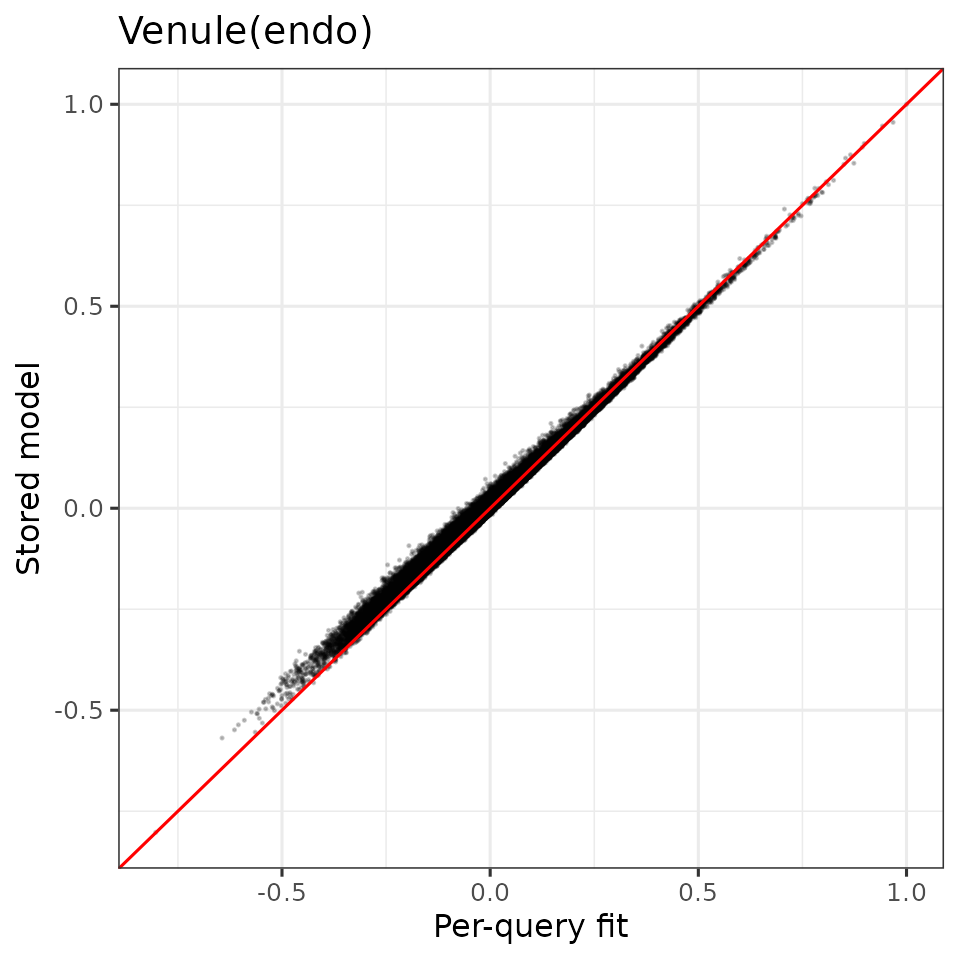

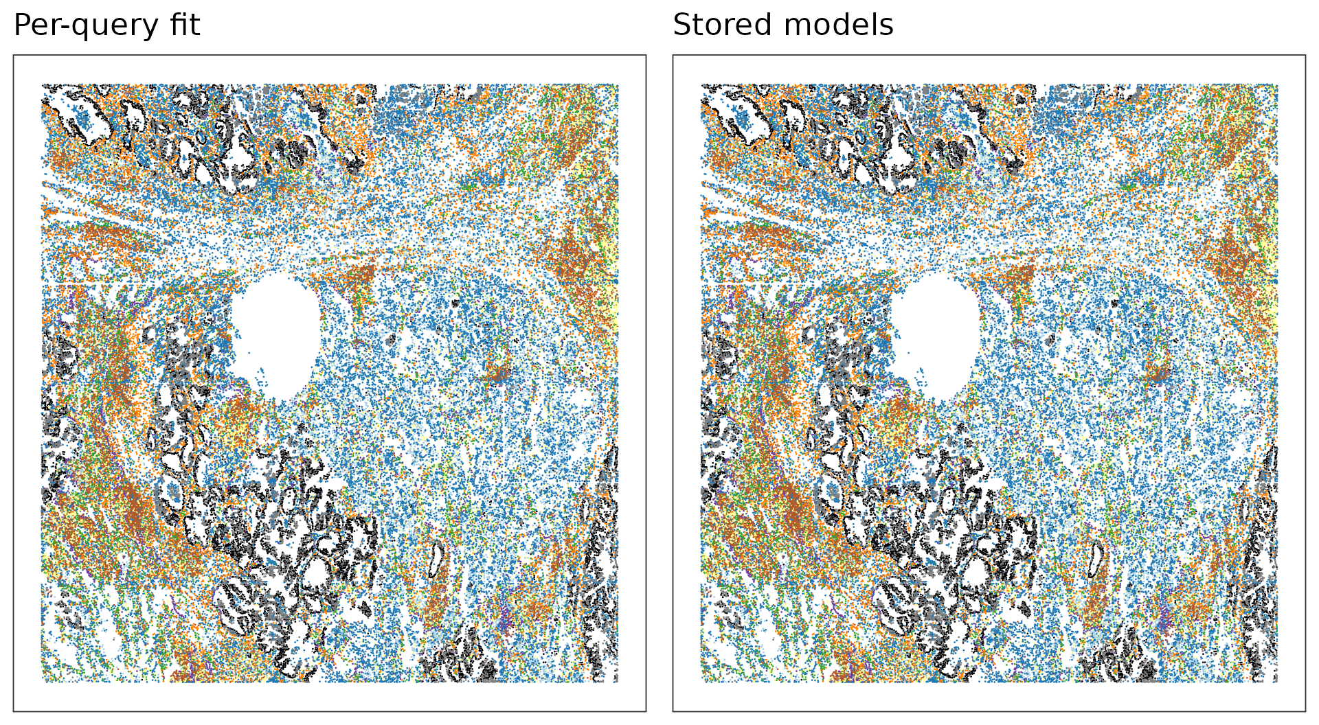
Next we find spatial niches with both sets of scores, with the settings of the CosMx vignette, and compare them with the adjusted Rand index (ARI; 1 for identical clusterings, about 0 for unrelated ones). Niche numbers are arbitrary, so the stored-model niches are renamed after the per-query niche that they overlap most. The Hartigan-Wong k-means of findNiches() warns that its quick-transfer stage reached its step limit, as in the CosMx vignette; these warnings are hidden here.

niche_args <- list(
  n_niches = 9, ncomp = 25,
  kmeans_algorithm = "Hartigan-Wong", kmeans_nstart = 50L, kmeans_iter = 200L,
  seed = 94863
)
niches_of <- function(scores) {
  reducedDim(query, "PhiSpace") <- scores
  sub("Niche_", "", do.call(findNiches, c(list(query), niche_args))$spatial_niches)
}
niches_query <- niches_of(scores_query)
niches_model <- niches_of(scores_model)

ari <- function(a, b) {
  tab <- table(a, b)
  pairs <- function(x) sum(choose(x, 2))
  expected <- pairs(rowSums(tab)) * pairs(colSums(tab)) / choose(sum(tab), 2)
  (pairs(tab) - expected) / ((pairs(rowSums(tab)) + pairs(colSums(tab))) / 2 - expected)
}
ari(niches_query, niches_model)

## [1] 0.9671335

# Match niches by their overlap, largest first
overlap <- table(niches_model, niches_query)
rename <- setNames(rep(NA_character_, nrow(overlap)), rownames(overlap))
for (k in order(overlap, decreasing = TRUE)) {
  i <- rownames(overlap)[(k - 1) %% nrow(overlap) + 1]
  j <- colnames(overlap)[(k - 1) %/% nrow(overlap) + 1]
  if (is.na(rename[i]) && !(j %in% rename)) rename[i] <- j
}
niches_model <- unname(rename[niches_model])
table(stored = niches_model, per_query = niches_query)

##       per_query
## stored     1     2     3     4     5     6     7     8     9
##      1 10194    20    16   119     3     3     1    14     0
##      2    30  5747    14    13     1     1     1    78     0
##      3     4     9 11172    42     0    26     4    26     0
##      4    45     2    37 28947    11    37     4   278     0
##      5     2     0     1    26  9091     2    10     6    77
##      6     3     0    21    57     1 10295     3    15     0
##      7     2     0     5     9     6     9  2186     5     2
##      8    22    22    59    61     2    39     4 11296     0
##      9     0     0     0     0   121     0     1     0  7642

nicheCols <- c(
  "1" = "#FF7F00", "2" = "#33A02C", "3" = "#B15928", "4" = "#1F78B4",
  "5" = "gray50", "6" = "#A6CEE3", "7" = "#6A3D9A", "8" = "#FFFF99", "9" = "black"
)
query$niche_query <- niches_query
query$niche_model <- niches_model
ggpubr::ggarrange(
  VizSpatial(query, "sdimx", "sdimy", colBy = "niche_query", ptSize = 0.5,
             legend.position = "none") +
    scale_colour_manual(values = nicheCols) + ggtitle("Per-query fit"),
  VizSpatial(query, "sdimx", "sdimy", colBy = "niche_model", ptSize = 0.5,
             legend.position = "none") +
    scale_colour_manual(values = nicheCols) + ggtitle("Stored models"),
  ncol = 2
)

Models for a known panel

If the panel of the queries is known when the model is trained, train on its genes with genes. Such a model needs no new selection, and gives the same scores as the per-query fit.

panel_models <- lapply(
  ref_list, trainPhiSpace,
  phenotypes = YtrainName, refAssay = "log1p", genes = rownames(query)
)
scores_panel <- reducedDim(PhiSpace(panel_models, query), "PhiSpace")
max(abs(scores_panel - scores_query))

## [1] 0

The choice between the two kinds of model is a trade-off. A model for a known panel is small and reproduces the per-query fit exactly, but suits only that panel. A whole-transcriptome model suits any query, at a small cost in agreement. A larger candidate pool (nfeatPool) gives the model more panel genes to select from, at the cost of model size: on these data, nfeatPool = 5000 raised the share of cells with the same top label from 96% to 98%, and made the four model files 2.9 GB instead of 0.8 GB.

Check the preprocessing of the query

A model can only give correct scores for a query that is preprocessed like its reference. Before scoring, predict() and PhiSpace() compare the query values with a summary of the reference values stored in the model, and warn if they look different. Here, the raw counts of the query are scored by mistake.

raw_counts <- suppressMessages(predict(models$endo, query, assay = "counts"))

## Warning: The query may be preprocessed differently from the reference of the
## model (Lung fibrosis, endo): the non-zero query values are all integers (raw
## counts?), the reference values are not. Preprocess the query as the reference
## (logTransf(use_log1p = TRUE) of counts).

The check cannot detect every difference. For example, counts normalised to different library sizes can pass it. Record the preprocessing in the model (preprocessing), and apply it to every query.

Save the results

Save the scores and niches; the website build checks them.

qs_save(
  list(
    scores_model = scores_model,
    niches_model = niches_model,
    niches_query = niches_query,
    cors = cors,
    agreement = agreement,
    niche_ari = ari(niches_query, niches_model),
    panel_max_abs_diff = max(abs(scores_panel - scores_query)),
    model_genes = vapply(models, function(m) length(m$selectedFeat), integer(1)),
    candidate_genes = vapply(models, function(m) nrow(m$stats$XtX), integer(1))
  ),
  paste0(dat_dir, "output/StoredModels_results.qs2")
)

Jiadong Mao

2026-10-13